The Dickey-Fuller test is a statistical test used to assess the null hypothesis that a unit root is present in an autoregressive model. 

History of Dickey-Fuller Test

The test was developed in the early 1970s by David A. Dickey and Wayne Fuller, and has since become one of the most widely used tests for determining stationarity in a time series.  

Put simply, this test determines whether or not there exists a unit root present in a particular time series dataset by testing whether the data follows a random walk. If it does not, then the null hypothesis is rejected and it can be concluded that the data contains some kind of pattern or structure.

How to carry out Dickey-Fuller Test?

In order to carry out the Dickey-Fuller Test, one must first formulate an autoregressive (AR) model which captures all relevant features of the dataset under consideration. The AR model essentially models an observed time series as being composed of previous values plus some random noise. 

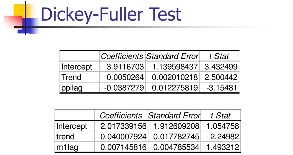
Once this model has been formulated, then it can be tested using the Dickey-Fuller Test, which involves fitting an ordinary least squares (OLS) regression on lagged values of the dependent variable. 

If this OLS regression produces statistically significant results, then it can be concluded that there is a unit root in the data and hence stationarity is rejected. Although originally designed for stationary time series datasets, the Dickey-Fuller Test has been extended and applied to nonstationary datasets as well with varying degrees of success. 

Advantages and Disadvantages

One key advantage of using this approach when dealing with nonstationary time series datasets is that it does not require any kind of trend or seasonality effects to be explicitly modeled upfront – this makes it more useful for many cases where such information may not be available beforehand. 

Additionally, since no prior assumptions need to be made about the underlying data distribution, this also allows for greater flexibility when dealing with nonstationary datasets compared to other methods like differencing or smoothing techniques which typically assume certain distributions upfront. 

Advantages of the Dickey-Fuller test include its ease of use, widespread applicability, and ability to handle a variety of different time series data. In addition, it allows for the incorporation of variables such as trends and seasonality, making it a powerful tool for forecasting and modeling economic variables. 

However, the Dickey-Fuller test also has a number of disadvantages. For one, it assumes that the underlying data is normally distributed, which may not always be the case in practice. 

Additionally, it can be subject to relatively high rates of false positives, particularly in smaller sample sizes. Finally, the Dickey-Fuller test cannot be used to test for the presence of more than one unit root, limiting its usefulness in certain situations. 

Conclusion

Overall, while not infallible due to its reliance on certain underlying assumptions about linearity and homoscedasticity within the dataset being tested; nonetheless, the Dickey-Fuller Test remains a highly effective tool for assessing stationarity in both stationary and nonstationary datasets due its ability to provide reliable statistical tests results without requiring any pre-defined assumptions about how certain aspects of these datasets should look like upfront – making it particularly useful when working with unfamiliar or untested datasets.